R Basics

Jonas, Pietro & Hauke

Before we start

If you haven’t done so already, please install R as well as RStudio now:

Outline

Session 1

In this session we will

make sure R & RStudio are up and running on all of your machines,
show why we like R,
introduce you to RStudio’s User Interface,
demonstrate some basic concepts and data structures.

Session 2

Read in and export data
Explore your data

Exercise & Break

Manipulate data
Analyze data

Session 3

Visualize data

Exercise & Break

Analysis Template: putting everything together
R6 intro (?)

Exercise & Time for Questions

Welcome to Session 1

Why we like R

Scripts vs. WYSIWYG (Excel or SPSS)

Analyses conducted in R are transparent, easily shareable, and reproducible. This helps not only others to run and understand your code but also your future selves.

Open Source

R is 100% free of charge and as a result, has a huge support community. it means that a huge community of R programmers will constantly develop an distribute new R functionality. It also means that you find a lot of help online as others ran into the same problems as you do.

Versatility

Yes, R is not Python. You can still use it to do a lot of stuff. If you can imagine an analytic task, you can almost certainly implement (and automate) it in R.

RStudio

RStudio helps you write R code. You can easily and seamlessly organize and combine R code, analyses, plots, and written text into elegant documents all in one place.

Examples & Use Cases

R & RStudio

RStudio is an integrated development environment (IDE) for R. It helps the user to effectively use R by making things easier with features such as:

Syntax highlighting,
Code completion,
Smart indentation,
Work spaces (more on that later), etc.

RStudio GUI

Opening RStudio, you will see four window panes:

bottom left: The Console executes code. You can use it to test code that is not saved.
upper left: The Source opens your scripts, markdown documents or notebooks. It is the one you’ll use the most as it allows you to write and save both comments and code. You have to actively run the code, though.
upper right: The Environment Pane displays the objects (e.g. data, variables, custom functions) you can access in your current memory.
bottom right: This pane shows you many different, yet important, tabs. You can browse your directory, view plots, get help and see installed packages.

Exercise

Create a script and save it.

Use comments

You can make comments using hashtags #.
Text behind # will not be evaluated.
You can use this to annotate your code or
to comment out code blocks you don’t need currently.

# calculate a sum that equals 4
2 + 2 # + 99

[1] 4

Sections

You can also use # some title ----- to create foldable sections in your scripts

Use comments

#
# Dear programmer:
# When I wrote this code, only god and I knew how it worked.
# Now, only god knows it!
#
# Therefore, if you are trying to optimize this routine
# and it fails (most surely), please increase this counter
# as a warning for the next person
#
# total_hours_wasted_here = 254
#

Vamos!

Operators

In the most simple form, R is an advanced calculator. Operators are symbols you know from any other program (Excel, etc.), such as + or -.

Operation	Description
x + y	Addition
x - y	Subtraction
x * y	Multiplication
x / y	Division
x ^ y	Exponentiation
x %/% y	Integer Division
x %% y	Remainder

Algebra

2+2
2 * 4
2^4
2 + (2 * 3) ^ 2
(1 + 3) / 2 + 45
13 %/% 3
13 %% 5

Exercise

What does Integer Division (line 6) and Remainder (line 7) actually mean? Run these lines and try to find out while tweaking the numbers a little.

Assign Values to Objects

R can keep several objects in memory at the same time
To distinguish them, objects have names.
Objects are assigned with <- or = (we recommend the former).

Don’t

Pretending 13 %% 5 was some important intermediate result that you’ll need later on, you shouldn’t run the same operation over and over again.

13 %% 5
# [1] 3
(13 %% 5) * 2
# [1] 6

Instead, assign an object (result) and refer to that one.

result <- 13 %% 5
result * 2
# [1] 6

Assign Values to Objects

Why <-

There is a general preference among the R community for using <- for assignment. This has at least two reasons:

Compatibility with old versions.
Ambiguity of = because it is used in other contexts (functions) as well.

Shortcuts

Mac: press option & -
Windows: press Alt & -

Assign Values to Objects

To inspect the objects you have just created you can call them.

result
# [1] 3

Alternatively, you can take a look into your Environment. Do you remember where to find it?

Naming

Conventions

Variable and function names should be lowercase.
If your code requires constants, use uppercase names.
Use an underscore _ to separate words within a name.
Strive for names that are concise and meaningful (this is not easy!).

# Good
day_one
day_1
VAT

# Bad
first_day_of_the_month
dayone
value_added_tax_constant

Case Sensitivity

Uppercase and lowercase letters are treated as distinct.

A <- 12
a <- 42
a == A

# [1] FALSE

Warning

Importantly, be careful to not reassign an object unintentionally.

a <- log(42)
a
# [1] 3.73767

# imagine to do some stuff in between...
# ...forgot about your object...
# ...and that you want to create another object called "a".

a <- 40 + 2
a
# [1] 42

Warning

Where possible, avoid using names

of special characters,
existing functions and
existing variables.

Doing so will cause confusion for the readers of your code.

# Bad
T <- FALSE
c <- 10
mean <- function(x) sum(x)

Note

Also, try to avoid special symbols such as +, for example. If you really need them, you can escape them using the back tick `

Data Types

There are many different data types. Today, we will focus on the most basic ones:

Data Type	Example
Numeric	`42`
Character	`"forty two"`
Logical	`TRUE`

Tip

Use class() to identify data types. class(42) will return numeric, for instance.

Changing Data Types

You will run into situations where R does not interpret data the way you want it. For instance, if R interprets the value 3 as "3", that is, as a character while it should be a numeric.

Luckily, R offers functions for these situations:

as.character(3)

[1] "3"

as.numeric("3")

[1] 3

as.logical(0)

[1] FALSE

as.logical(1)

[1] TRUE

# does not work: as.numeric("three")

Vectors

We can combine objects with the c() command to create a vector.

The documentation says:

The default method combines its arguments to form a vector. All arguments are coerced to a common type which is the type of the returned value […].

a     <- c(1, 2, 3)
cntry <- c("CH", "FR", "NL", "DK")
test  <- c(1, 3, 5, "seven")

Exercise

What does All arguments are coerced to a common type actually mean? Hint: use class() for a & test.

Break

please answer the survey if you haven’t done so already

x <-  3
x < - 3

Boolean Algebra

Description

A Boolean expression is a logical statement that is either TRUE or FALSE.

3 < 4
3 >= 4
3 == 4
3 != 4

!TRUE
TRUE | FALSE
TRUE & FALSE

Note

You can also abbreviate TRUE and FALSE with T and F.

Boolean Algebra

Operation	Description	Output
x < y	Less than	TRUE if x is smaller than y. FALSE otherwise
x <= y	Less or equal than	TRUE if x is smaller or equal than y. FALSE otherwise
x > y	Greater than	TRUE if x is greater than y. FALSE otherwise
x >= y	Greater or equal than	TRUE if x is greater or equal than y. FALSE otherwise
x == y	Exactly equal to	TRUE if and only if x is equal to y. FALSE otherwise
x != y	Not equal to	TRUE if and only if x is not equal to y. FALSE otherwise

!x	Negation	TRUE if x is equal to FALSE or 0. FALSE otherwise
x \| y	OR	TRUE if x or y or both are TRUE . FALSE otherwise
x & y	AND	TRUE if and only if x and y are both TRUE . FALSE otherwise

Selecting

Let’s combine what we learned about vectors and Boolean algebra.

Exercise

Create a vector called countries that contains “CH”, “FR”, “NL” & “DK”.

Selecting

Tip

Show the vector’s first entry using countries[1].

Tip

Show whether the vector contains "EN" with "EN" %in% countries.

Tip

Show where the vector contains "DK" with match("DK", countries).

Functions

So far, you have seen several built-in functions: class() & c().

You can recognize a function either via class()¹ or by the parentheses.

To call a function, you have to provide some argument(s). The mean() function needs some sort of vector, for instance.

How to get Help?

Assume you want to learn how to use the mean() function.

?mean or help(mean)
Use stackoverflow

Packages

Packages are the fundamental units of reproducible R code. They include reusable R functions, the documentation that describes how to use them, and sample data.
The comprehensive R Archive Network currently features 18.694 packages.
The majority of packages is quite niche-specific.
To get started, we’ll show you how to install Tidyverse, an opinionated collection of R packages designed for data science. All packages share an underlying design philosophy, grammar, and data structures.

Using packages

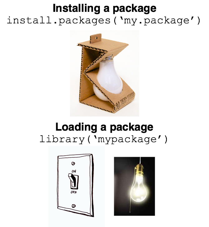
An R package is like a lightbulb. First you need to order it with install.packages(). Then, every time you want to use it, you need to turn it on with library()

# run this only once
install.packages("package_name")

# run this at the beginning of each session (if needed)
library(package_name)

Exercise

Your turn

Install tidyverse, which contains the lubridate package with a function called year()
get the documentation for the following function: Sys.Date()
execute Sys.Date() %>% year()
Load lubridate
execute Sys.Date() %>% lubridate::year()

Note

install.packages("package_name")

library(package_name)

Find installed Packages

Remember that the bottom right panel has a Packages tab? Let’s inspect it.

The %>% Operator

Let’s apply some functions. Can you guess the outcome?

paste0(round(sqrt(82), digit = 2), " is your result!")

We can do the same using %>%:

sqrt(82) %>% round(digit = 2) %>% paste0(" is your result!")

Proof

To prove that there is no difference between the two outcomes, we compare them:

paste0(round(sqrt(82), digit = 2), " is your result!") == sqrt(82) %>% round(digit = 2) %>% paste0(" is your result!")

[1] TRUE

Your turn

create a vector called vec containing 1, 2, 3, 99
calculate the mean() using both methods
round the results (one digit) and assign it to objects called res1 & res2
show that both are equal

vec <- c(1, 2, 3, 99)
res1 <- mean(vec) %>% round(digits = 1)
res2 <- round(mean(vec), digits = 1)
res1 == res2

[1] TRUE

Exercise

Generate three objects

my_pi should contain the number pi (try out the command pi)
a vector, called a, should contain the numbers 1 to 3
b should be the multiplication of 1*pi, 2*pi 3*pi

Environment

We can see all objects currently in our work space by typing ls().
You can remove objects using rm()

ls()
rm(a)

# What do you think is going to happen here?
rm(list = ls())

You should actually apply this.

Delete unused elements

This makes your environment easier to read and saves some memory.

Start with a fresh session

This forces you to

document all used objects in your script and
load all packages you are using.

It, thus, makes your code more reproducible and less likely to break.

Don’t!

Exercises

create a new variable called my_num that contains 6 numbers
multiply my_num by 4
create a second variable called my_char that contains 5 character strings
combine the two variables my_num and my_char into a variable called both (hint: you can use the c() function)
what is the length of both (hint: try the length() function)
what class is both?
divide both by 3, what happens?
create a vector with elements 1 2 3 4 5 6 and call it x
create another vector with elements 10 20 30 40 50 and call it y
what happens if you try to add x and y together? why?
append the value 60 onto the vector y (hint: you can use the c() function)
add x and y together
multiply x and y together. pay attention to how R performs operations on vectors of the same length.

Bonus: Scripts, Markdown & Project

Scripts are a great way to document how you analyzed your data.
Like a recipe, scripts make it easy (for you and others) to reproduce your process exactly.
You can also use RMarkdown, which allows you to blend code chunks with text.¹
To make your code even more organized and reproducible, use R Projects.

Resources

swirl is a great start as it teaches you R interactively, at your own pace, and right in the R console! Run the following code to get started.

install.packages("swirl") # install this package once
library(swirl)
siwrl()

Resources

Resources we found helpful creating the slides:

Welcome to Session 2

Recap Session 1 - What we did

Setting up R
Get to know the UI
Objects, classes, operations
Packages

Any experienced difficulties? Anything we should repeat?

Recap: Packages in R

Beyond base R’s core functions, packages provide additional functionality for (almost) all of your problems.

Some of the most widely-used packages are included in the tidyverse collection install.packages("tidyverse") and library(tidyverse) brings you most of the functions you will need (at this point):

For example:

manipulate data: dplyr
tidy data: tidyr
visualize data: ggplot2

There are many more packages available

Recap: Practical Advice

Pitfall

Failing to load a package is a common error source - one you can easily avoid by loading everything you need right at the start.

This is how the very beginning of your code could look like:

setwd("/Users/haukeroggenkamp/Documents/coursework/bootcampR") #set your working directory
#install.packages("ggplot2") # only needed for installing once
#install.packages("tidyverse") # only needed for installing once
library(tidyverse) # load package

Overview Session 2 - Working with data

Read in and export data
Explore your data

Exercise & Break

Manipulate data
Analyze data

Exercise & Time for Questions

What’s next: We need some data to work with!

Reading in and storing data

Data can come in various file formats, e.g., .csv, .xlsx, .sav etc. We can read all these files into our environment.

For that, we always specify the location path to the local data source (and we directly assign our data to an object called data)

Reading in

data <- read.table(file = "data/raw/student_experiment.csv",
                   sep = ";", 
                   header = TRUE) # you need to adapt this to your working directory file path

Saving

write.table(x    = data, 
            file = "data/processed/student_experiment_processed.csv") # writes the final dataframe as a .csv file into your specified directory

Good to know

We recommend text files (.csv or .txt), however, there are packages for reading in other file formats (haven, foreign or rio).

Exploring data I/II

You should know how your data is structured before processing it and R has some neat functions to do that:

head(data) shows the first few rows of your data
names(data) shows the column or variable names of your data
view(data) shows the entire data in a new window

head(data)
names(data)

  lfdn external_lfdn tester dispcode lastpage
1    2             0      0       31  6061029
2    4             0      0       31  6061029
3   11             0      0       31  6061029
4   13             0      0       31  6061029
5   14             0      0       31  6061029

 [1] "lfdn"          "external_lfdn" "tester"        "dispcode"     
 [5] "lastpage"      "quality"       "duration"      "expectation"  
 [9] "r_experience"  "interest_data"

Exploring data II/II

To get a feeling for your data, you can investigate summary statistics:

summary(data$rent)

   Min. 1st Qu.  Median    Mean 3rd Qu.    Max.    NA's 
  400.0   532.5   640.0   814.8   712.5  3000.0       1

rstatix::get_summary_stats(data, rent, type="five_number")

# A tibble: 1 × 7
  variable     n   min   max    q1 median    q3
  <chr>    <dbl> <dbl> <dbl> <dbl>  <dbl> <dbl>
1 rent        12   400  3000  532.    640  712.

We can calculate the mean rent of this course individually:

mean(data$rent)

[1] NA

How about the course’s gender distribution?

table(data$gender) # 1 = male, 2 = female


1 2 
8 5

Or the mean shoe size by gender?

stats::aggregate(shoesize ~ gender, data, FUN = mean)

  gender shoesize
1      1   43.125
2      2   37.800

Break (10min) and Exercises

Load the survey data and assign it to a dataframe object named df (if not done so already)
How many rows and columns does df contain?
Calculate simple summary statistics for the df
Calculate the standard error for the variable shoesize

Manipulate your data

Some important functions from dplyr:

select Choose which columns to include.
filter Filter which rows to include.
arrange Sort the data, by size for continuous variables, by date, or alphabetically.
group_by Group the data by a categorical variable.
n() Count the number of records. Here there isn’t a variable in the brackets of the function, because the number of records applies to all variables.
mutate Create new column(s) in the data, or change existing column(s).
rename Rename column(s).
bind_rows Append one data data frame to another, combining data from columns with the same name.

Manipulate: `select` and `filter`

data %>% 
  select(gender, rent) # show just the specified columns

  gender rent
1      2   NA
2      2 3000
3      1  950

data %>%
  filter(gender==1 & shoesize ==44) %>% select(gender, shoesize) # show just males with a shoesize of 44

  gender shoesize
1      1       44
2      1       44
3      1       44

Recap: %>%(pipe) operator

%>% makes code easier to write and read. It works similar to a + sign and is an integral part of the tidyverse syntax

Manipulate: `arrange` and `n`

data %>% 
     filter(gender == 2 & rent >= 900) %>% # only females with rent above 900CHF
     arrange(desc(rent)) %>% # sort by descending rent 
        select(gender, rent) # show only the columns gender and rent

  gender rent
1      2 3000

data %>%
  filter(gender == 2) %>% # only female
  summarise(
    n = n()) # number of instances written in new column with name n

  n
1 5

summarise()

summarise() reduces multiple values down to a single summary.

Manipulate: `group_by`

data %>%
  group_by(gender) %>% # group by gender
  summarise(
    n = n(), # counte the instances and write in column named n
    avg_height = mean(height, na.rm = TRUE),
    avg_rent = mean (rent, na.rm = TRUE)) # calculate the mean height and write in avg_height column

# A tibble: 2 × 4
  gender     n avg_height avg_rent
   <int> <int>      <dbl>    <dbl>
1      1     8       182.     616.
2      2     5       158.    1212

Removing NAs

na.rm allows you to exclude instances of missing value. This helps to prevent error messages. But check why is that data missing!

Manipulate: `mutate` and `rename`

data %>% 
  mutate(gender, sq_height = height ^ 2) %>% # adds variable that is a function of existing ones
  select(gender, sq_height) # ashow only the columns gender and the new variable

  gender sq_height
1      2     23104
2      2     21025
3      1     34225
4      1     32400
5      1     34225

data %>% 
  rename(
    cost_for_living = rent, # renames a column (new name = old name)
    )

  lfdn external_lfdn tester dispcode lastpage
1    2             0      0       31  6061029
2    4             0      0       31  6061029
3   11             0      0       31  6061029
4   13             0      0       31  6061029
5   14             0      0       31  6061029

Put it all together

data %>%  # Start with the data 
               filter(r_experience <= 6) %>% # Oonly those with R experience below 6
               group_by(gender) %>%    # Group by gender
               summarise( 
                        age.mean = mean(age),      # Define first summary...
                        height.mean = median(height), # you get the idea...
                        n = n()) %>% # How many are in each group?
        select(age.mean, height.mean, n)

# A tibble: 2 × 3
  age.mean height.mean     n
     <dbl>       <int> <int>
1     22.9         185     7
2     27.4         154     5

Help

It can sometimes be hard to understand what a command is doing with the data. Tidy data tutor visualizes what is happening to your data in every code step which is extremely helpful.

Break (10 min) and Exercises

Build a new dataframe called df_demographics that contains just the demographic information from our survey data
Rename the gender column to sex column in this dataframe
Calculate the mean age by gender in this dataframe
Calculate the logarithmic rent of all male participants of the AIBS course and store it in a column named log_rent

Advanced: Join two dataframes

inner_join: To keep only rows that match from the data frames, specify the argument all=FALSE. To keep all rows from both data frames, specify all=TRUE.
left_join: To include all the rows of your data frame x and only those from y that match.

Example: Calculate year born of members of this class:

age_table <- read.csv(file = "data/raw/age_table.csv") # read in age table from directory
data_new <- left_join(data, select(age_table, c(X2022_after, year_born)), by = c("age" = "X2022_after")) # perform join to get the birthyear
data_new %>% select(age, year_born) %>% filter(age<24) # show the results

  age year_born
1  22      2000
2  22      2000
3  21      2001
4  23      1999
5  22      2000
6  23      1999
7  22      2000

Advanced: Long to wide dataformat

data_long to data_wide

ncol(data) # number of columns in long format

[1] 55

data_wide <- pivot_wider(data = data, names_from = age, values_from = height)
ncol(data_wide) # number of columns in wide format

[1] 60

The arguments to pivot_longer():

data: Data object
names_from: Name of column containing the new column names
values_from: Name of column containing values

Reverse Way

The reverse way from wide to long format via pivot_wider

Analyze your data: Statistical Analysis with R

You (R) can do a lot:

t-Test
ANOVA
Regression
Structural Equation Models
Multilevel Models
Machine Learning Models
Bayesian Statistics
…

Stats 1: t-Test

Recap: Mean comparisons (>= 2 groups)

t.test(formula = rent ~ gender, data = data, alternative = 'two.sided') # base R


    Welch Two Sample t-test

data:  rent by gender
t = -0.99236, df = 3.0711, p-value = 0.3926
alternative hypothesis: true difference in means between group 1 and group 2 is not equal to 0
95 percent confidence interval:
 -2481.5  1290.0
sample estimates:
mean in group 1 mean in group 2 
         616.25         1212.00

rstatix::t_test(data = data, formula = rent~gender, alternative = "two.sided") # the same works with other packages, here `rstatix`

# A tibble: 1 × 8
  .y.   group1 group2    n1    n2 statistic    df     p
* <chr> <chr>  <chr>  <int> <int>     <dbl> <dbl> <dbl>
1 rent  1      2          8     5    -0.992  3.07 0.393

Notice the difference in the code?

Caution

There are similar functions t.test and t_test from different packages using different syntax

Stats 2: Analysis of Variance

Recap: Mean comparisons (> 2 groups)

Is there a difference in XYZ?

data$course <- as.factor(data$education) # this ensures our factor to be of the right class
summary(aov(formula = rent~education, data = data))

            Df  Sum Sq Mean Sq F value Pr(>F)
education    1  573944  573944   1.176  0.304
Residuals   10 4882419  488242               
1 Beobachtung als fehlend gelöscht

Caution

The underlying grouping variable needs to be as.factor. Always check first!

anova(lm(formula = rent~education, data = data)) # Same analysis possible by running a linear model and wrapping the `anova` function for omnibus test

Analysis of Variance Table

Response: rent
          Df  Sum Sq Mean Sq F value Pr(>F)
education  1  573944  573944  1.1755 0.3037
Residuals 10 4882419  488242

Stats 3: Regression

Recap: Relationship between two (or more) variables

Is there a relationship between height and shoesize?

summary(lm(formula = shoesize~height, data = data)) # runs a linear model and provides statistical summary


Call:
lm(formula = shoesize ~ height, data = data)

Residuals:
    Min      1Q  Median      3Q     Max 
-2.6840 -1.2487 -0.3436  0.9486  4.0510 

Coefficients:
            Estimate Std. Error t value Pr(>|t|)    
(Intercept)  6.96106    5.93868   1.172 0.265895    
height       0.19729    0.03421   5.767 0.000125 ***
---
Signif. codes:  0 '***' 0.001 '**' 0.01 '*' 0.05 '.' 0.1 ' ' 1

Residual standard error: 1.871 on 11 degrees of freedom
Multiple R-squared:  0.7514,    Adjusted R-squared:  0.7288 
F-statistic: 33.26 on 1 and 11 DF,  p-value: 0.0001252

Remember: Live-saving advice: How to get help when stuck?

?lm() will immediately provide you with Help in the panel
CRAN documentations and Cheat Sheets are a comprehensive source of support (hard to read at the beginning)
Google is your friend: Chance is high that someone else had a very similar question to yours on stackoverflow.com; try different search terms and exact language

Jump in: Time for exercising

Basic Exercises

Regress rent on height and shoesize
Calculate the mean difference between r_experience by class and perform a t-test
Do r_experience and interest_data correlate?

Advanced exercises:

Add a column containing the shoe size converted to the US system and correlate US with EU shoesize
Hint: load the shoesizes dataset from Canvas and look for potential information that might match with our data

Prepare your questions for tomorrow’s Q&A

Specific to your projects?
Put them on Canvas or bring them to the lecture

Welcome to Session 3

Belated Session 2 Bonus

Recap

Tidyverse

You have seen that there are many functions such as filter(), select(), etc. in the dplyr package. Please name other functions the package provides.

Recap

Resource

Visit tidydatatutor.com and scroll down a little. You’ll find helpful visualizations over there.

Base R

We’ll use tidyverse functions as a reference today and explain how to do similar stuff in base R, that is, without loading any packages.

To illustrate this, we’ll first load some data.

data("USArrests")
head(USArrests)

           Murder Assault UrbanPop Rape
Alabama      13.2     236       58 21.2
Alaska       10.0     263       48 44.5
Arizona       8.1     294       80 31.0
Arkansas      8.8     190       50 19.5
California    9.0     276       91 40.6
Colorado      7.9     204       78 38.7

Back to vectors

Remember how we selected items in (one-dimensional) vectors?

vec <- c('a', 'b', 'c', 'd')

vec[2]

Back to vectors

Remember how we selected items in (one-dimensional) vectors?

vec <- c('a', 'b', 'c', 'd')

vec[2]
# [1] "a"

vec[c(1, 3)]

Back to vectors

Remember how we selected items in (one-dimensional) vectors?

vec <- c('a', 'b', 'c', 'd')

vec[2]
# [1] "a"

vec[c(1, 3)]
# [1] "a" "c"

vec[c(FALSE, FALSE, FALSE, TRUE)]

Back to vectors

Remember how we selected items in (one-dimensional) vectors?

vec <- c('a', 'b', 'c', 'd')

vec[2]
# [1] "b"

vec[c(1, 3)]
# [1] "a" "c"

vec[c(FALSE, FALSE, FALSE, TRUE)]
# [1] "d"

Here is a more practical example where we want to rename the column UrbanPop.

names(USArrests) # this is a vector
# [1] "Murder"   "Assault"  "UrbanPop" "Rape" 

# vector ------- condition -------------------- re-assignment
names(USArrests)[names(USArrests) == 'UrbanPop'] <- 'urban_pop'

names(USArrests)
# [1] "Murder"   "Assault"  "urban_pop" "Rape"

Select Cells

We can do the same thing with (two dimensional) data frames without using the tidyverse:

USArrests[1, 2]
# [1] 236

USArrests[1, c(1, 2)]
#         Murder Assault
# Alabama   13.2     236

Filter Data

With dplyr::filter() we were able to display all the rows that match a certain condition, such as Murder > 10.

How shall we do this with base R?

USArrests$Murder > 10
# [1]  TRUE FALSE FALSE FALSE FALSE ...

Filter Data

With dplyr::filter() we were able to display all the rows that match a certain condition, such as Murder > 10.

How shall we do this with base R?

USArrests$Murder > 10
# [1]  TRUE FALSE FALSE FALSE FALSE ...

USArrests[USArrests$Murder > 10,]
#                Murder Assault UrbanPop Rape
# Alabama          13.2     236       58 21.2
# Florida          15.4     335       80 31.9
# Georgia          17.4     211       60 25.8
# ...              ...      ...       .. ...
# Texas            12.7     201       80 25.5

Select Columns

We talked about this yesterday.

USArrests$Murder
# [1] 13.2 10.0  8.1  8.8 ...

USArrests[, 'Murder']
# [1] 13.2 10.0  8.1  8.8 ...

USArrests[[1]]
# [1] 13.2 10.0  8.1  8.8 ...

Select Assalt Statistics

Inspect the data and look for the Assault Variable. Then select it using all of the three options displayed above.

Exercise 1

Please show all the states with an above-median number of Assaults.

               Murder Assault UrbanPop Rape
Alabama          13.2     236       58 21.2
Alaska           10.0     263       48 44.5
Arizona           8.1     294       80 31.0
Arkansas          8.8     190       50 19.5
California        9.0     276       91 40.6
Colorado          7.9     204       78 38.7
Delaware          5.9     238       72 15.8
Florida          15.4     335       80 31.9
Georgia          17.4     211       60 25.8
Illinois         10.4     249       83 24.0
Louisiana        15.4     249       66 22.2
Maryland         11.3     300       67 27.8
Michigan         12.1     255       74 35.1
Mississippi      16.1     259       44 17.1
Missouri          9.0     178       70 28.2
Nevada           12.2     252       81 46.0
New Mexico       11.4     285       70 32.1
New York         11.1     254       86 26.1
North Carolina   13.0     337       45 16.1
Rhode Island      3.4     174       87  8.3
South Carolina   14.4     279       48 22.5
Tennessee        13.2     188       59 26.9
Texas            12.7     201       80 25.5
Wyoming           6.8     161       60 15.6

Exercise 1

Please show all the states with an above-median number of Assaults.

USArrests[USArrests$Assault > median(USArrests$Assault), ]

               Murder Assault UrbanPop Rape
Alabama          13.2     236       58 21.2
Alaska           10.0     263       48 44.5
Arizona           8.1     294       80 31.0
Arkansas          8.8     190       50 19.5
California        9.0     276       91 40.6
Colorado          7.9     204       78 38.7
Delaware          5.9     238       72 15.8
Florida          15.4     335       80 31.9
Georgia          17.4     211       60 25.8
Illinois         10.4     249       83 24.0
Louisiana        15.4     249       66 22.2
Maryland         11.3     300       67 27.8
Michigan         12.1     255       74 35.1
Mississippi      16.1     259       44 17.1
Missouri          9.0     178       70 28.2
Nevada           12.2     252       81 46.0
New Mexico       11.4     285       70 32.1
New York         11.1     254       86 26.1
North Carolina   13.0     337       45 16.1
Rhode Island      3.4     174       87  8.3
South Carolina   14.4     279       48 22.5
Tennessee        13.2     188       59 26.9
Texas            12.7     201       80 25.5
Wyoming           6.8     161       60 15.6

Exercise 2

What is the average number of murders in these states?

[1] 11.175

Exercise 2

What is the average number of murders in these states?

mean(USArrests[USArrests$Assault > median(USArrests$Assault), 'Murder'])

[1] 11.175

Recap Session 2

Read in and export data
Explore your data
Manipulate data
Analyze data

Any experienced difficulties? Anything we should repeat?

Recap: import and export data

Reading in

data <- read.table("data/raw/student_experiment.csv", sep = ";", header = T) # you need to adapt this to your working directory file path

Saving

write.table(data, "data/processed/student_experiment_processed.csv") # writes the final dataframe as a .csv file into your specified directory

Recap: Exploring data

head(data) shows the first few rows of your data
names(data) shows the column or variable names of your data
view(data) shows the entire data in a new window

Overview Session 3

Visualization
Organize your project
Analysis Template: putting everything together
Questions

Why visualization?

Data visualization is the practice of representing data in a graphical form (e.g. plots). This is a powerful way to visualize information in a way that is understandable to the majority of the audience (and impress your professors when presenting the empirical project). For this reason it is crucial to select the type of visualization that best fits our data and our goal!

Ggplot - grammar of graphics

Ggplot is a powerful package for creating visualizations. Its strength relies on the underlying Grammar of Graphics, a set of rules of combining independent elements into a graphical representations.

Elements of grammar of graphics

Data: variables mapped to aesthetic features of the graph.
Geoms: objects/shapes on the graph.
Stats: statistical transformations that summarize data,(e.g mean, confidence intervals).
Scales: mappings of aesthetic values to data values. Legends and axes visualize scales.
Coordinate systems: the plane on which data are mapped on the graphic.
Faceting: splitting the data into subsets to create multiple variations of the same graph (paneling).

Ggplot bulding blocks

ggplot() initializes the coordinate system of our visual representation. It takes as input the dataset of interest.
geom_*() specifies the type of visualization. It needs a mapping argument which maps the variables from the dataset to the objects on the plot.
aes() is assigned to the mapping argument. It takes as argument the values corresponding to the x and y axis, as well as other plot-specific characteristics (e.g., color, size, fill,…)
Additional functions can be added to to specify labeling and thematic characteristics (ggtitle(),xlab(),ylab(),theme()).

Remember: It is always possible to get help regarding these function by running ?functionName

Type of data visualization I/III

Univariate visualizations

Univariate graphical representation visualize the distribution of data from a single continuous or discrete variables.

Bar plot: representation of categorical categorical data.
Histograms, distribution plot and box plot: representation of the distribution of numerical data.

bar plot (left) histogram with kernel distribution (right)

ggplot(diamonds) + geom_bar(mapping=aes(x=cut))
ggplot(diamonds, aes(x = depth)) + 
        geom_histogram(aes(x=depth, y = ..density..),
                 colour = 1, fill = "white") +
        geom_density()

Type of data visualization II/III

Bivariate visualizations

Bivariate visual analysis shows relationship between two variables. It is important to select the correct visualization type according to the variables analysed:

Continuous v Continuous
Discrete v Discrete
Discrete v Continuous

Type of data visualization II/III

Bivariate visualizations (Continuous v Continuous)

ggplot(diamonds) +
  geom_point(aes(
           x = carat, 
           y = price))

ggplot(diamonds,aes(x = carat, 
           y = price)) +
  geom_point() +
  geom_smooth(method = "lm")

Type of data visualization II/III

Bivariate visualizations (Discrete v Discrete)

ggplot(diamonds) + 
  geom_bar(aes(x = color, 
           fill = cut), position = "stack")

ggplot(diamonds) + 
  geom_bar(aes(x = color, 
           fill = cut), position = "dodge")

Type of data visualization II/III

Bivariate visualizations (Discrete v Continous)

ggplot(diamonds, 
       aes(x = color, 
           y = price)) +
  geom_boxplot() +
  labs(title = "Salary distribution by rank")

ggplot(diamonds, 
       aes(x = price, 
           fill = color)) +
  geom_density(alpha = 0.4) +
  labs(title = "Salary distribution by rank")

Type of data visualization III/III

Multivariate visualizations

Multivariate presentation show the relationship of 3 or more variables. There are two main approaches grouping and faceting.

Grouping represents the data on a single plot when the x and y axis represent two variables and the third is displayed through visual elements such as colors, dot shape, size, etc.
Faceting simply include different plot in one single visualization.

Type of data visualization III/III

Multivariate visualizations (Grouping)

ggplot(diamonds) +
  geom_point(aes(x = carat, 
           y = price, color=color, shape=cut))

ggplot(diamonds) +
  geom_point(aes(x = carat, 
           y = price, color=color, size=depth))

Type of data visualization III/III

Multivariate visualizations (Faceting)

price ($1000) histogram by color and cut

# plot salary histograms by rank and sex
ggplot(diamonds, aes(x = price/1000)) +
  geom_histogram(color = "white",
                 fill = "cornflowerblue") +
  facet_grid(cut ~ color)

Resources

Easy to read book chapter
A full book
And another one
List of geoms
As always: Stackoverflow

Organize your project

Create a new folder called BootcampR
Create a R script file
Set your working directory to your_path_to/BootcampR
Create a folder called data
Create two subdirectories: data/raw and data/preprocessed
Move the file mtcars.csv into data/raw

Organize your project

Create a new folder called BootcampR
Create a R script file
Set your working directory to your_path_to/BootcampR

setwd('`your_path_to/BootcampR`')

Create a folder called data

dir.create('data')

Create two subdirectories: data/raw and data/preprocessed

dir.create('data/raw')
dir.create('data/preprocessed')

Move the file mtcars.csv into data/raw

Break

Download the mtcars.csv file from canvas :)

Analysis Template: putting everything together

Packages

Task

Install and load the following packages:

ggplot
ggcorrplot
dplyr
tidyverse

Solution

install.packages('tidyverse')
install.packages('ggplot')
install.packages('dplyr')
install.packages("ggcorrplot")

library(ggplot2)
library(dplyr)
library(ggcorrplot)
library(tidyverse)

Constants

This is the place where you assign constants, e.g. the Swiss VAT:

VAT <- 0.077 # Swiss VAT (7.7%)

Remember that we use a different naming convention for constants, i.e. uppercase letters.

REMEMBER: Working Directories

getwd() # identify your current directory
setwd() # adjust it if needed

Read Data

Task

Import the mtcars.csv file into an object called mtcars_df

Solution

Ideally, you have a folder called data that contains two subfolders:

raw from where you read the original data &
processed where you store the data after you have transformed it

mtcars_df <- read.csv(file = 'data/raw/mtcars.csv',
                sep  = ',')

Data Dictionary

variable	description
mpg	Miles/(US) gallon
cyl	Number of cylinders
disp	Displacement (cu.in.)
hp	Gross horsepower
drat	Rear axle ratio
wt	Weight (1000 lbs)
qsec	1/4 mile time
vs	Engine (0 = V-shaped, 1 = straight)
an	Transmission (0 = automatic, 1 = manual)
gear	Number of forward gears
carb	Number of carburetors

Data Exploration

Task

List all the variables in the dataset
Create a new dataset called new_mtcars which includes only the following columns: mpg, hp, wt, vs, gear
Calculate the summary statistics of the new dataset
Visualize the bar plot of vs and distribution density of wt
Calculate and visualize a correlation matrix

Solution

names(mtcars_df)
 
new_mtcars <- mtcars_df  %>% select(mpg, hp, wt, vs, gear)

summary(new_mtcars)

#ggplot(new_mtcars) + geom_bar(mapping=aes(x=vs))
ggplot(new_mtcars, aes(x = wt)) + 
        geom_histogram(aes(x=wt, y = ..density..),
                 colour = 1, fill = "white") +
        geom_density()

corr <- round(cor(new_mtcars), 1)
ggcorrplot(corr, lab=TRUE)
#ggcorrplot(corr, lab=TRUE, type='lower')

Data Transformation

Task

Generate a new variable called hp_wt which is the ration of hp and wt
Remove the variables hp and wt

Solution

new_mtcars$hp_wt <- new_mtcars$hp/new_mtcars$wt
new_mtcars <- subset(new_mtcars, select=-c(wt,hp))

Save Data

Task

Save the new dataset in data/processed

Solution

There are different formats you can use. CSV is the most compatible format.

write.csv(x = new_mtcars,
          file = 'data/processed/transformed_data.csv')

Data Analyses

Task

Train a linear regression model that predicts car consumption given engine type (VS or Straight), number of gears and power-to-weight ratio and show the summary statistics
Visualize the linear relationship between consumption and power-to-weight ratio
Predict consumption for a new car with straight engine, 6 gears and a power-to-weight ratio of 36.1

Solution

car_mpg_lm <- lm(mpg ~ vs + gear + hp_wt, data = new_mtcars)
summary(car_mpg_lm)

ggplot(new_mtcars,aes(x = hp_wt, 
           y = mpg)) +
  geom_point() +
  geom_smooth(method = "lm") 
new_data <- data.frame(vs=1,
                  gear=6,
                  hp_wt = 36.1)

pred = predict(car_mpg_lm, newdata = new_data)
pred

Thank you

and good luck on your empirical project :)

R Basics

Before we start

Outline

Session 1

Session 2

Session 3

Welcome to Session 1

Why we like R

Examples & Use Cases

R & RStudio

RStudio GUI

Use comments

Use comments

Vamos!

Operators

Algebra

Assign Values to Objects

Assign Values to Objects

Assign Values to Objects

Naming

Data Types

Changing Data Types

Vectors

Break

Boolean Algebra

Boolean Algebra

Selecting

Selecting

Functions

How to get Help?

Packages

Using packages

Exercise

Find installed Packages

The %>% Operator

Exercise

Environment

Exercises

Bonus: Scripts, Markdown & Project

Resources

Resources

Welcome to Session 2

Recap Session 1 - What we did

Any experienced difficulties? Anything we should repeat?

Recap: Packages in R

Recap: Practical Advice

Overview Session 2 - Working with data

What’s next: We need some data to work with!

Reading in and storing data

Exploring data I/II

Exploring data II/II

Break (10min) and Exercises

Manipulate your data

Manipulate: select and filter

Manipulate: arrange and n

Manipulate: group_by

Manipulate: mutate and rename

Put it all together

Break (10 min) and Exercises

Advanced: Join two dataframes

Advanced: Long to wide dataformat

Analyze your data: Statistical Analysis with R

Stats 1: t-Test

Stats 2: Analysis of Variance

Stats 3: Regression

Remember: Live-saving advice: How to get help when stuck?

Jump in: Time for exercising

Basic Exercises

Advanced exercises:

Prepare your questions for tomorrow’s Q&A

Welcome to Session 3

Belated Session 2 Bonus

Recap

Recap

Base R

Back to vectors

Back to vectors

Back to vectors

Back to vectors

Select Cells

Manipulate: `select` and `filter`

Manipulate: `arrange` and `n`

Manipulate: `group_by`

Manipulate: `mutate` and `rename`